
spatial factor multi-species occupancy model with NSW WildCount Data between 2012-2021
Methodology
- Data Collection and Preprocessing
Occurrence Data: Consolidated species occurrence records from BioNets (2012-2021) filtered to the "Wild Count Fauna" dataset.
Extracted key fields: species names, coordinates, dates, and location identifiers.
1.1. About the WildCount Dataset WildCount examined trends in the occurrence of animals and was one of the first monitoring programs in the world to assess a broad suite of animals at such a large scale. The data generated identified changes in occupancy to understand if animals are in decline, increasing or stable and ultimately guide on-ground management.
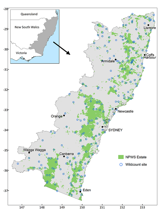
The 200 WildCount camera sites are located in 146 national parks and reserves across eastern New South Wales. Every year, between 2012 and 2021, 4 motion-sensing cameras were placed at each site between February and June. Cameras were left in the field for a minimum of 2 weeks and captured over 250,000 images each year.
1.2. About diet and community of Spotted-tailed quoll Based on previous studies on spotted-tailed quoll, we identified 26 species from 12 family that are the primary mammal prey items/competitor of spotted-tailed quoll, and is available inside the WildCount Dataset:
family.name [1] "Canidae" "Dasyuridae" "Felidae" "Leporidae" "Macropodidae" "Muridae"
[7] "Peramelidae" "Petauridae" "Phalangeridae" "Potoroidae" "Pseudocheiridae" "Vombatidae"
We used family as modelling unit in this study because the aim of this study is to predict realistic STQ distribution based on species interaction: STQ interact with these species via predator-prey relationship, and they do not have specific hunting preferences but the prey size. Fortunetly, the species inside each family in this study have similar body size (e.g. Phalangeridae = brustail possum = medium size mammals), which make grouping them more ecological sense to STQ. Grouping them into family as modelling unit also smoothing out rare species and help increase data availablity Reducing the total number of modelling unit also help reduce complexity of the model (26 -> 12) Predator species is not impacted as they belongs to their own family. (i.e. Canidae = fox, Dasyuridae = STQ, felidae =CAT) *note dingos are not included in the study as they have no record
We downloaded all the data between 2012-2021 for the mentioned family, then combine them into single dataset.
1.2. Extracting survey location WildCount data on the BioNet do not contain direct locations of their trap sites. We are currently requesting exact camera trap locations from the NSW government but did not receive any reply yet. Aussming each trap location will have at least one record of any of our study species(family) between 2012-2021, we extracted all the unique coordinatesin the dataset. The dataset contain 827 unique coordinates, rough match with the official WildCount Dataset description (200 sites * 4 cameras = 800 trap locations). We also visually inspect and compare the coordinates in our dataset with the published map (https://www2.environment.nsw.gov.au/sites/default/files/2024-09/wildcount-map.png), based on similar pattern observed. We believe the coordinates of our dataset is a good proxies of the real trap sites.
1.3. Replicates
To create occupancy model, we grouped records into two-year intervals (replicate), creating five temporal replicates (2012–2013 = 1, ..., 2020–2021 = 5),
matching the turnover of STQ (three years ideal but this will leave one year out).
THIS FORMED THE BASIC STRUCTURE OF THE MODEL
- Detection-Nondetection Data Structure
Formatted data into a 3D array y with dimensions:
Species (N = 12),
Sites (J = 827),
Replicates (K = 5)
Entries: 1 (detection), 0 (non-detection), or NA (unsampled site-replicate).
- Covariate Preparation
Detection Covariates:
Survey effort: BioNet Dataset do not have traping effort recorded. Official description mentioned that each trapping period spanned at least 2 weeks. So in here we assume for each occurrence record, the max/min trapping start date is +- 14 days, which approxiametly equal to one month. Therefore, for each records, we assume the whole month has been surveyed and conut that as 1 survey effort , and we sum up the number of unique sampling months per site-replicate, scaled and formatted into a matrix aligned with y.
detection covariates in the model must be site/replicate specific, which we can't include species specific detection covariates in it (e.g. common/rare species, body size, etc.)
Occurrence Covariates: Extracted from raster layers at site coordinates:
Bioclimatic variables (bio5, bio12; mean temperature of warmest quarter, annual precipitation): We used CHELSA model, the model has consistent data across three period (2011-2040, 2041-2070, 2071-2100) with 6 GCM models (GFDL, IPSL, MPI, MRI, UKESM) and 3 scenarios (ssp126, ssp370, ssp585) We will run each each years-model-scenarios and take the mean occurrence probability for each year-scenario To address multicollinearity and ecological relevance for prioritizing bioclimatic variables for STQ, we did a pearson correlation analysis to all the variables Initial analysis revealed high correlation (|r| > 0.7) among temperature and precipitation variables (e.g., Bio1, Bio5, Bio12, Bio17). Variables were grouped into clusters based on correlation, and one representative variable per cluster was retained to avoid overfitting and ensure model robustness.
Bio5 (Max Temperature of Warmest Month) was prioritized over other temperature variables (e.g., Bio1, Bio10) because it directly quantifies extreme heat events, which is the direct impact of climate change. STQ is sensitive to therma extremes. Also, other mean variables will smooth out the extreme.
Bio12 (Annual Precipitation) was selected over seasonal precipitation metrics (e.g., Bio13, Bio17) as it reflects total annual moisture availability, a foundational requirement for maintaining the quolls’ core habitats (e.g., rainforests, wet sclerophyll forests). moisture context is more related to quoll's habitat but not their survival requirement as they consume water from prey item. Rationale: Quolls are absent from arid regions, and declining annual precipitation (Bio12) under climate change will fragment and degrade moist forest habitats critical for denning and foraging. Climate Change Context: Long-term drying trends in southeastern Australia threaten to reduce annual rainfall below thresholds necessary for quoll persistence.
Anthropogenic factors (road density, population density): We use road density and population density as proxies for anthropogenic disturbance. This are choosen because they will keep relatively unchanged or available for projection (population density). We initially planned to create an index combining the two variables ut decided later to leave that for the model.
(forest loss? fragmentation index?)
Environmental predictor (depth of regolith).
Other variables to included? (Forest cover, foliage cover)
We enabled Quadratic terms for bioclimatic variables and depth of regolith, assuming species occurrences will peak in certain range. We keep anthropogenic factors linear, assuming species will love to away from human as far as possible.
- Spatial and Temporal Alignment
We Removed sites with missing covariates (1 site excluded, i.e. 826 sites remains).
Ensured alignment of y, covariates, and coordinates matrix.
- Model Specification
Integrated spOccupancy Framework:
Occupancy Formula: Community-level effects of scaled covariates with quadratic terms: ~ scale(bio5) + I(scale(bio5)^2) + scale(bio12) + I(scale(bio12)^2) + scale(roadLength) + scale(pd_mean) + scale(der) + I(scale(der)^2)
Detection Formula: Scaled survey effort: ~ scale(effort)
Spatial Process: Exponential covariance with NNGP approximation (15 neighbors) for computational efficiency.
- Model Execution
Tested with 250 MCMC iterations (10 batches x 25 iterations) to validate data structure and priors.
Full model would extend to robust iterations for convergence (e.g., 25,000 iterations post-burn-in).
- Output Analysis
Evaluated community-level parameter summaries (posterior means, credible intervals) to infer species-environment relationships.
Key Innovations
Temporal binning to address sparse annual data.
Multi-species spatial occupancy framework accommodating detectability and rare species.
Integration of anthropogenic and bioclimatic predictors for holistic habitat modeling.
We assess MCMC convergence using the following three tools included inside the packages:
- Gelman-Rubin Rhat diagnostic (indication of convergence)
- Effective Sample Size (indication of mixing)
- Visual assessment of trace plots