








A Python package to efficiently model active- and passive-particle transport in flowing rivers.
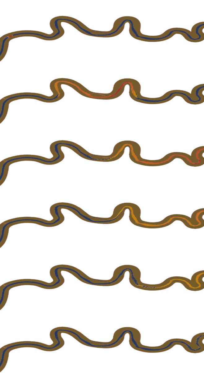
This package advects conservative flow tracers (a.k.a. passive particles) with the fluid velocity and displaces them with stochastic diffusion due to fluid turbulence over discrete time steps. It tracks particles under a Lagrangian frame of reference as they move through a curvilinear 2- or 3-D hydrodynamic mesh. Users may customize particle subclasses to implement additional active particle motions, e.g. channel-bed adjacent sinusoidal vertical motion to simulate the preferred swimming patterns of white sturgeon larvae (McDonald and Nelson, 2021). Since version 0.1.0 the package also tracks particles along 1D river networks routed by pywatershed, described in the section below.
As the total simulation duration, the size of the mesh, or the number of particles increases, so too do the computational resources used in the simulation (real-world time, memory, etc.). fluvial-particle uses the efficient array storage and operator methods of NumPy and VTK to update particle positions. Simulation results are written to hierarchical data format (HDF5) files using the h5py package, which allows writing and compression of terabytes of data.
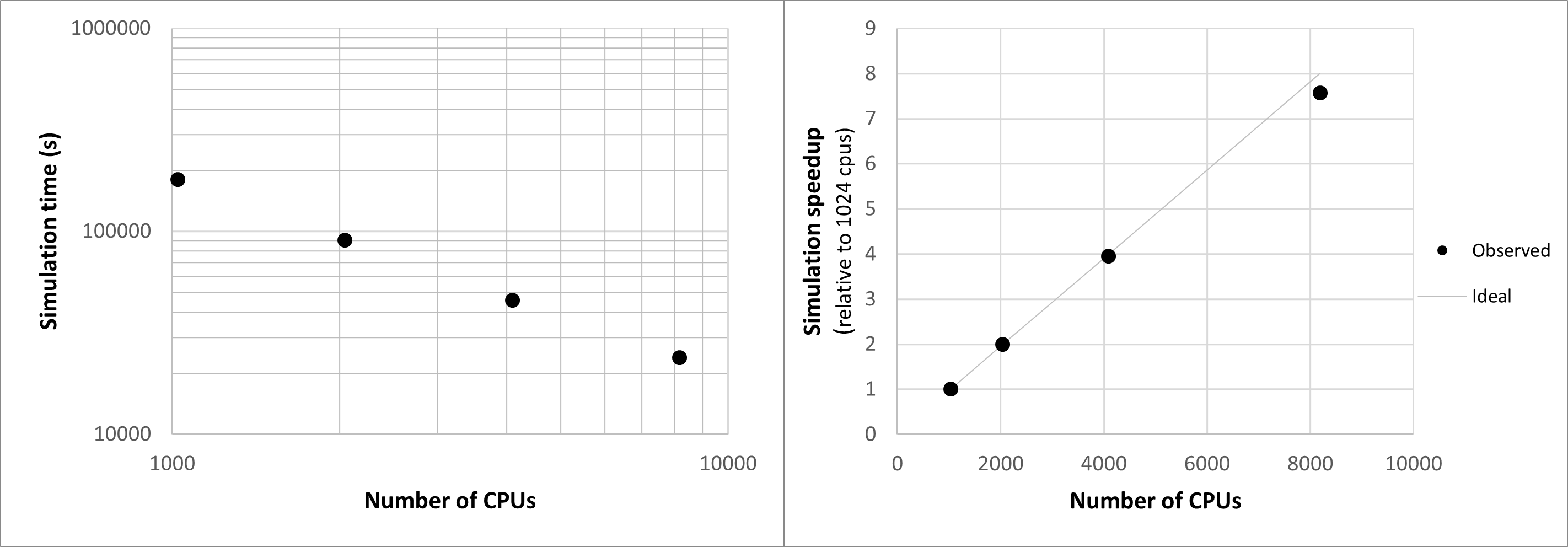
Prohibitively large or long simulation problems can be made tractable with the highly scalable fluvial-particle package. The mpi4py package enables massively-parallel execution mode to simulate millions or billions of particles (or more!). A strong-scaling test simulation of 227 particles on the Kootenai River over many thousands of CPUs shows that MPI-enabled fluvial-particle scales well, as shown in the figure below.
- Lagrangian particle tracking on 2D and 3D hydrodynamic meshes (VTK
.vtsand.vtk, NumPy.npz), with active-particle subclasses for behaviors such as larval swimming and settling - 1D river-network particle tracking driven by pywatershed network hydraulics exports (new in 0.1.0, see below)
- Parallel execution with MPI through mpi4py
- TOML settings files, a notebook API (
run_simulation/SimulationResultsandrun_network_simulation/NetworkResults), and HDF5/XDMF, VTP/PVD, and NetCDF output
This package uses uv for fast dependency installation and hatchling for building. It is recommended to use a conda environment.
First, create the fluvial-particle conda environment using the environment.yml file:
conda env create -f environment.yml
conda activate fluvial-particle
Next, install uv if you don't have it already:
pip install uvThen use uv to install the package and its dependencies:
uv pip install -e .The success of the installation can be tested with pytest:
pytest testsDirections on invoking fluvial-particle from the command line can be found in the docs.
Version 0.1.0 adds a second solver, fluvial_particle.network, for passive transport along a river network rather than across a 2D/3D mesh. It reads the network hydraulics NetCDF export written by pywatershed (pywatershed.utils.export_network_hydraulics): reach topology, daily flow, velocity, depth, width and shear velocity, and optional map polylines. Particles advect exactly along reaches, cross junctions carrying the unused part of the time step, disperse with a Fischer coefficient built from the exported hydraulics, and exit at outlets with their arrival times recorded. Sources are mass loadings (slugs, constant or tabulated loading, or concentration curves), and the results give arrival-time distributions, map positions, and concentration on sub-reach bins.
A minimal settings file:
[network]
hydraulics_file = "drb_network_hydraulics.nc"
start_time = "1979-03-01"
end_time = "1979-04-01"
dt = 900.0
output_interval = 3600.0
particle_mass = 1.0

[[network.sources]]
reach_id = 4205
form = "slug"
time = 0.0
mass = 1000.0
Run it from the command line or from Python:
fluvial_particle_network settings.toml -o output
mpiexec -n 4 fluvial_particle_network_mpi settings.toml -o output
from fluvial_particle import run_network_simulation
res = run_network_simulation("settings.toml", "output", seed=42)
print(res.summary())
arrivals = res.arrival_histogram(outlet=4205, bin_seconds=3600)
concentration = res.concentration(time=-1, bin_length=500.0)See the network documentation and the demo notebooks: notebooks/network-drb-demo.ipynb (Delaware River Basin: headwater slugs, a continuous loading, breakthrough at Trenton, a map animation) and notebooks/network-chain-dispersion-demo.ipynb (a uniform chain compared with the analytical advection-dispersion solution).
- Environments with conda plus uv for fast installs; packaging with hatchling
- Test automation with Nox; testing with pytest and Coverage.py, reported to Codecov
- Linting, formatting, and pre-commit hooks with Ruff; static type checking with mypy
- Security checks with Bandit and pip-audit
- Continuous integration, releases, and labels with GitHub Actions, Release Drafter, and GitHub Labeler
- Documentation with Sphinx (autodoc, napoleon, MyST) on Read the Docs
- Version management with bump-my-version
Contributions are very welcome. To learn more, see the Contributor Guide.
Distributed under the terms of the CCO 1.0 license, Fluvial Particle is free and open source software.
If you encounter any problems, please file an issue along with a detailed description.
This project was generated from hillc-usgs's Pygeoapi Plugin Cookiecutter template.
This package is based on the model described by McDonald & Nelson (2021), A Lagrangian particle-tracking approach to modelling larval drift in rivers, Journal of Ecohydraulics, 6(1) 17-35.